Scenario 24 - 29
License
Overview

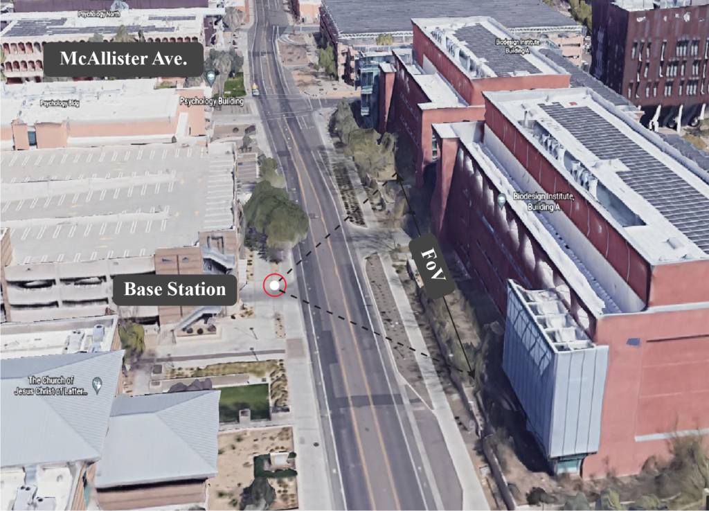
Illustration of the data collection scenario/location, where Unit 1 (TX) and Unit 2 (RX) were deployed on the two sides of the street. The right subfigure shows the equipment used in our dataset collection.
Scenarios 24 – 29 are collected in an outdoor wireless environment representing a two-way city street. We adopt the DeepSense Testbed 3 and add a synchronized LiDAR sensor. The scanning range of the LiDAR is 16 meters and the motor spin frequency is 10Hz. The testbed is deployed in this environment where the two units are placed on the opposite sides of the street. The transmitter (Unit 2) constantly transmits using one antenna element of the phased array to realize omnidirectional transmission. The receiver continuously scans the surrounding environment using a receive mmWave beam steering codebook of 64 beams and by measuring the receive power with each beam. The testbed collects data samples at a rate of 10 samples/s. The LiDAR at Unit 1 continuously scans the environment. Each data sample has multiple modalities including an RGB image and a LiDAR 360-degree point cloud, both collected by Unit 1. Please refer to the detailed description of the testbed presented here.
McAllister Ave: It is a two-way street with 2 lanes, a width of 10.6 meters, and a vehicle speed limit of 25mph (40.6 km per hour. It is worth mentioning here that since this is a city street, vehicles of various sizes and travel speeds pass in both directions. This creates a diverse pool of blockages for the LOS link between the transmitter and receiver, which results in diverse received power maps (i.e., diverse power fluctuations across all 64 beam over time instances) and a diverse dataset.
Scenarios 17-22 are outdoor wireless environments representing a two-way city street. The DeepSense Testbed 3 is deployed in this environment where the two units are placed on the opposite sides of the street. The transmitter (Unit 2) constantly transmits using one antenna element of the phased array to realize omnidirectional transmission. The receiver continuously scans the surrounding environment using a receive mmWave beam steering codebook of 64 beams and by measuring the receive power with each beam. The testbed collects data samples at a dynamic rate ranging from 6 to 12 samples/s. The average sampling rate is 10 samples/s. Each data sample includes an RGB image and a 64-element receive power vector, both collected by Unit 1. Please refer to the detailed description of the testbed presented here.
McAllister Ave: It is a two-way street with 2 lanes, a width of 10.6 meters, and a vehicle speed limit of 25mph (40.6 km per hour. It is worth mentioning here that since this is a city street, vehicles of various sizes and travel speeds pass in both directions. This creates a diverse pool of blockages for the LOS link between the transmitter and receiver, which results in diverse received power maps (i.e., diverse power fluctuations across all 64 beam over time instances) and a diverse dataset.

Collected Data
Overview
Number of Data Collection Units: 2 (using DeepSense Testbed #3)
Total Number of Data Samples: 500000
Scenario-wise Data Samples: Scenario 24: 40000 || Scenario 25: 80000 || Scenario 26: 80000 || Scenario 27: 100000 || Scenario 28: 100000 || Scenario 29: 100000
Data Modalities: RGB images, 64-dimensional received power vector, GPS locations
Sensors at Unit 1: (Stationary Receiver)
- Wireless Sensor [Phased Array]: A 16-element antenna array operating in the 60 GHz frequency band and receives the transmitted signal using an over-sampled codebook of 64 pre-defined beams
- Visual Sensor [Camera]: The main visual perception element in the testbed is an RGB-D camera. The camera is used to capture RGB images of 960×540 resolution at a base frame rate of 30 frames per second (fps)
- Position Sensor [GPS Receiver]: A GPS-RTK receiver for capturing accurate real-time locations for the stationary unit 1
- LiDAR Sensor [2D laser scanner]: This system provides the range and angle data of objects within its range of view. This system covers a maximum range of 16 meters around the master component and it operates at a maximum scan rate of 10 Hz
Sensors at Unit 2: (Mobile Transmitter)
- Wireless Sensor [Phased Array]: A stationary 60 GHz mmWave transmitter. The transmitter (Unit 2) constantly transmits using one antenna element of the phased array to realize omnidirectional transmission
- Position Sensor [GPS Receiver]: A GPS-RTK receiver for capturing accurate real-time locations for the stationary unit 2
| Testbed | 3 |
|---|---|
| Instances | Scenario 24: 40000 || Scenario 25: 80000 || Scenario 26: 80000 || Scenario 27: 100000 || Scenario 28: 100000 || Scenario 29: 100000 |
| Number of Units | 2 |
| Data Modalities | RGB images, 64-dimensional received power vector, GPS locations, LiDAR point cloud |
| Unit1 | |
| Type | Stationary |
| Hardware Elements | RGB camera, mmWave phased array receiver, GPS receiver, LiDAR |
| Data Modalities | RGB images, 64-dimensional received power vector, GPS locations, LiDAR point cloud |
| Unit2 | |
| Type | Stationary |
| Hardware Elements | mmWave omni-directional transmitter, GPS receiver |
| Data Modalities | GPS locations |
Data Visualization
Download
Please login to download the DeepSense datasets
How to Access Scenario Data?
Step 1. Download Scenario Data
Step 2. Extract the scenarioX.zip file
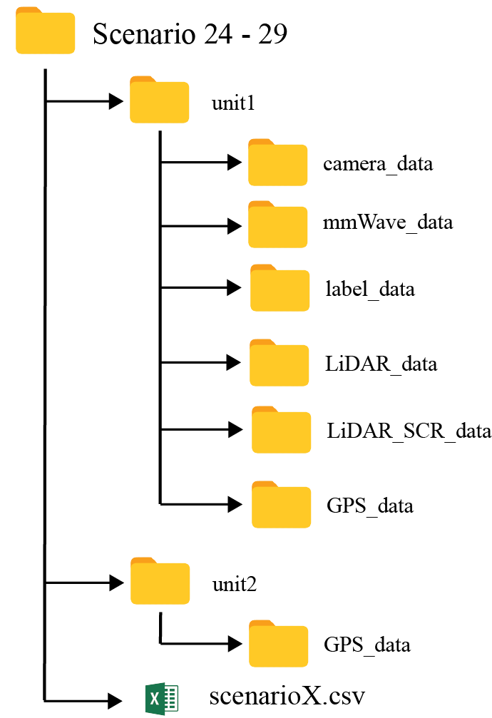
Scenario X folder consists of three sub-folders:
- unit1: Includes the data captured by unit 1
- unit2: Includes the data captured by unit 2
- resources: Includes the scenario-specific annotated dataset, data labels, and other additional information. For more details, refer to the resources section below.
The scenario X folder also includes the “scenario X.csv” file with the paths to all the collected data. For each coherent time, we provide the corresponding visual, wireless, and GPS data.

Resources
What are the Additional Resources?
Resources consist of the following information:
- data labels: The labels comprises of the ground-truth link blockage status
- additional information: Includes the scenario-specific additional data. Details of the information is provided below
Visual Data Annotations
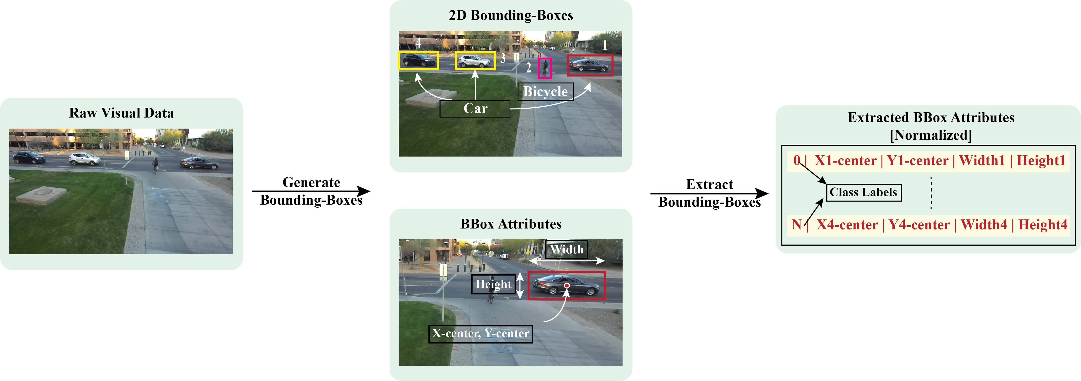
After performing the post-processing steps presented here, we generate the annotations for the visual data. Using state-of-the-art machine learning algorithms and multiple validation steps, we achieve highly accurate annotations. In this particular scenario, we provide the coordinates of the 2D bounding box and attributes for each frame.
We, also, provide the ground-truth labels for ‘8’ object classes as follows: ‘1’: person || ‘2’: bicycle || ‘3’: car || ‘4’: motorcycle || ‘5’: airplane || ‘6’: bus || ‘7’: train || ‘8’: truck
We follow the YOLO format for the bounding-box information. In the YOLO format, each bounding box is described by the center coordinates of the box and its width and height. Each number is scaled by the dimensions of the image; therefore, they all range between 0 and 1. Instead of category names, we provide the corresponding integer categories.

Data Labels
The label comprises of the ground-truth link-status manually annotated from the RGB images
- Ground-Truth Blockage: We utilize the RGB images and manually annotate the data samples with link-status labels. More specifically, a link-status label of ‘1’ is assigned to a time instance when the LOS link is blocked, and a label of ‘0’ otherwise.
- Ground-Truth Blockage: We utilize the RGB images and manually annotate the data samples with link-status labels.
Additional Information
We, further, provide additional information for each sample present in the scenario dataset. The contents of the additional data is listed below:
- index: It represents the sample number
- time_stamp[UTC]: This represents the time of data capture in “hr-mins-secs-ms” format
An example table comprising of the data labels and the additional information is shown below.
| index | unit1_rgb | unit1_pwr_60ghz | unit1_lidar | unit1_lidar_SCR | unit1_blockage | unit1_loc | unit2_loc | time_stamp[UTC] | seq_index |
|---|---|---|---|---|---|---|---|---|---|
| 1 | ./unit1/camera_data/image1_07_26_11.jpg | ./unit1/mmWave_data/mmWave_power_1.txt | ./unit1/LiDAR_data/lidar_data_1.mat | ./unit1/LiDAR_SCR_data/lidar_SCR_data_1.mat | ./unit1/label_data/label_1.txt | ./unit1/GPS_data/gps_location.txt | ./unit2/GPS_data/gps_location.txt | ['07-26-11-0'] | 1 |
| 2 | ./unit1/camera_data/image2_07_26_11.jpg | ./unit1/mmWave_data/mmWave_power_2.txt | ./unit1/LiDAR_data/lidar_data_2.mat | ./unit1/LiDAR_SCR_data/lidar_SCR_data_2.mat | ./unit1/label_data/label_2.txt | ./unit1/GPS_data/gps_location.txt | ./unit2/GPS_data/gps_location.txt | ['07-26-11-166'] | 1 |
| 3 | ./unit1/camera_data/image3_07_26_11.jpg | ./unit1/mmWave_data/mmWave_power_3.txt | ./unit1/LiDAR_data/lidar_data_3.mat | ./unit1/LiDAR_SCR_data/lidar_SCR_data_3.mat | ./unit1/label_data/label_3.txt | ./unit1/GPS_data/gps_location.txt | ./unit2/GPS_data/gps_location.txt | ['07-26-11-332'] | 1 |
| 4 | ./unit1/camera_data/image4_07_26_11.jpg | ./unit1/mmWave_data/mmWave_power_4.txt | ./unit1/LiDAR_data/lidar_data_4.mat | ./unit1/LiDAR_SCR_data/lidar_SCR_data_4.mat | ./unit1/label_data/label_4.txt | ./unit1/GPS_data/gps_location.txt | ./unit2/GPS_data/gps_location.txt | ['07-26-11-498'] | 1 |
| 5 | ./unit1/camera_data/image5_07_26_11.jpg | ./unit1/mmWave_data/mmWave_power_5.txt | ./unit1/LiDAR_data/lidar_data_5.mat | ./unit1/LiDAR_SCR_data/lidar_SCR_data_5.mat | ./unit1/label_data/label_5.txt | ./unit1/GPS_data/gps_location.txt | ./unit2/GPS_data/gps_location.txt | ['07-26-11-664'] | 1 |
| 6 | ./unit1/camera_data/image6_07_26_11.jpg | ./unit1/mmWave_data/mmWave_power_6.txt | ./unit1/LiDAR_data/lidar_data_6.mat | ./unit1/LiDAR_SCR_data/lidar_SCR_data_6.mat | ./unit1/label_data/label_6.txt | ./unit1/GPS_data/gps_location.txt | ./unit2/GPS_data/gps_location.txt | ['07-26-11-830'] | 1 |
| 7 | ./unit1/camera_data/image7_07_26_12.jpg | ./unit1/mmWave_data/mmWave_power_7.txt | ./unit1/LiDAR_data/lidar_data_7.mat | ./unit1/LiDAR_SCR_data/lidar_SCR_data_7.mat | ./unit1/label_data/label_7.txt | ./unit1/GPS_data/gps_location.txt | ./unit2/GPS_data/gps_location.txt | ['07-26-12-0'] | 1 |
| 8 | ./unit1/camera_data/image8_07_26_12.jpg | ./unit1/mmWave_data/mmWave_power_8.txt | ./unit1/LiDAR_data/lidar_data_8.mat | ./unit1/LiDAR_SCR_data/lidar_SCR_data_8.mat | ./unit1/label_data/label_8.txt | ./unit1/GPS_data/gps_location.txt | ./unit2/GPS_data/gps_location.txt | ['07-26-12-111'] | 1 |
| 9 | ./unit1/camera_data/image9_07_26_12.jpg | ./unit1/mmWave_data/mmWave_power_9.txt | ./unit1/LiDAR_data/lidar_data_9.mat | ./unit1/LiDAR_SCR_data/lidar_SCR_data_9.mat | ./unit1/label_data/label_9.txt | ./unit1/GPS_data/gps_location.txt | ./unit2/GPS_data/gps_location.txt | ['07-26-12-222'] | 1 |
| 10 | ./unit1/camera_data/image10_07_26_12.jpg | ./unit1/mmWave_data/mmWave_power_10.txt | ./unit1/LiDAR_data/lidar_data_10.mat | ./unit1/LiDAR_SCR_data/lidar_SCR_data_10.mat | ./unit1/label_data/label_10.txt | ./unit1/GPS_data/gps_location.txt | ./unit2/GPS_data/gps_location.txt | ['07-26-12-333'] | 1 |

